Gene Expression Inference with Deep Learning

Bioinformatics Application of Deep Learning Technology

Resource

We will discuss the following paper: Chen et al., Gene expression inference with deep learning. Bioinformatics. 2016 Jun 15;32(12):1832-9.  The paper is available here.

All figures shown here should be credited to the paper.

Introduction

The main goal of deep learning (DL) (or deep neural network - DNN) is feature learning, i.e., it finds a non-linear transformation function $\mathbf{z} = \phi(\mathbf{x})$ to project raw input feature $\mathbf{x}$ into new feature $\mathbf{z}$, hopefully the feature vectors in the Z space will be more linearly behaved, so that linear regression or logistic regression method performs better.  As DNN can theoretically model any function (see the DL Introduciton blog), we therefore can train a DNN; the parameters that give better predictions arguably has found a better approximation of $\phi$.  Chen et al. used a classical fully-connected DNN (basically is the black-box DNN model we imagined previously) for feature transformation and coupled with a traditional linear regression output layer.  I like this study, because its design is very clean, the paper is very readable and the conclusions are convincing.

Human genome contains about 20000 genes.  Genes are expressed at different levels within cells.  Different cell types, different life cycle stages, and different treatments all lead to changes in gene expression, the expression of genes controls what proteins to be expressed and at what level, which subsequently determines all the biological activities in and among cells.  So the expression level of 20k genes basically form a feature vector fingerprinting the cell status.  For example, to understand the effects of 1000 compounds, we would need to treat cells with each of compound and then measure 1000 gene expression profiles, one per compound.  As each expression profiling costs ${\rm $}500$, this is quite expensive.  In a previous work by NIH LINCS, it was proposed that gene expression data are highly redundant, therefore, one only needs to profile the expression values of a subset of 1000 landmark genes, called L1000; the expression values for the remaining genes can be computationally predicted.  Previously, for a given target gene $t$ to be predicted, linear regression is used and its expression is predicted based on:

$$\begin{equation} y_{i(t)} = \sum_{j=1}^{1000} w_j x_j + b_i, \end{equation}$$

where $x$ are the measured expression levels of L1000 genes.  However, in reality, gene expression is regulated through a non-linear system through the complicated interactions of molecular circuits.  Therefore the dependency of $y_i(t)$ on L1000 expressions must be a complicated non-linear function, this is where DNN shines compared to traditional machine learning methods.  The authors did exact this and showcase the power of DNN for feature transformation.

Results

D-GEX

A fully connected DNN is used as illustrated in the Figure below, called D-GEX (stands for Deep-Gene Expression).  A few details, first there are 943 *(not 1000) landmark genes, because the study uses three different data sets and some landmark and target genes are not included, as they are not contained in all three sets.  This also explains why there 9520 (not 20000) target genes in the future, as others do not have test data available for error/accuracy evaluation.  Second, there seems to be two DNNs, this is the memory requirements for predicting all 9520 genes is too much for a single GPU, therefore two GPUs had to be used; each was responsible for the predicting of 4760 (randomly allocated) genes.  For our purpose, we just need to consider this is one fully connected DNN with 943 inputs and 9520 outputs.

The authors have tested many different DNN hyperparameters, including number of hidden layers [1, 2, 3], number of neurons within each layer [3000, 6000, 9000].  It uses dropout regularization with values [0%, 10%, 25%].  It uses momentum optimization and Glorot weight initialization (all these concepts are explained in the Introduction blog).  These are the key ingredients and the author performed full grid search of the hyperparameter space formed by the combinations of layer count, layer size and dropout rate.

About 100k gene expression samples were retrieved from Gene Expression Omnibus (GEO) database, and was split into 80-10-10 training-validation-test datasets.  So the training matrix is $943 \times 88807$, the validation matrix is $943 \times 11101$ and the test matrix is $943 \times 11101$.  The loss function is defined as least-square error, as this is a regression problem:

$$\begin{equation} L= \sum_{t=1}^{T} \left[ \frac{1}{N} \sum_{i=1}^{N}{\left( y_{i(t)} - \hat{y}_{i(t)} \right)}^2 \right], \end{equation}$$

where the errors between the true values $y$ and the predicted values $\hat{y}$ were calculated and summed for all $T = 9520$ target genes and then summed over all $N$ training samples within a batch.  Typically $L$ is used to optimize network parameters $\theta$, one can define another accuracy function to measure the network performance, which is more interpretable and which is used to calculate validation and test errors (for the purpose of cross validation or early termination).  The accuracy function typically is not suitable for parameter optimization, where loss function has better gradient properties.  Here the error is defined intuitively as mean average error:

$$\begin{equation} MAE_{(t)}= \frac{1}{N^\prime} \sum_{i=1}^{N^\prime} \left\vert \left( y_{i(t)} - \hat{y}_{i(t)} \right)\right\vert. \end{equation}$$

Comparison

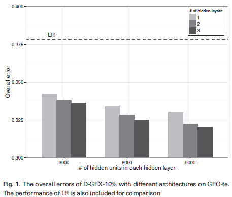
D-GEX was optimized and its performance obtained under various hyperparamters are shown in the figure below.  It says the best performance (the smallest overall error as determined based on Equation 3) was achieved with 3 9000-neuron layers and 10% dropout rate, i.e., the most complicated DNN structure (D-GEX-10%-9000X3).  The error 0.32 is significantly less (15.33% improvement) compared to the traditional linear regression (LR) method (the horizontal dashed line) (The figure is a bit misleading, its Y axis should have started from 0 instead of 0.3).

More performance data is shown in the table below.  It shows even a single-layer NN performs better than LR.  It also shows linear regression achieves error rate of 0.378, and regularization (either L1 or L2) did not really boost its performance.  This is understandable, as we have 88807 training samples and only 944 parameters to fit for a given target gene, overfitting should not be a concern.  The k-nearest-neighbor (KNN) method, a non-parametric method, performed the worst.

In the figure below, each point represents a gene, where the X axis is its prediction error based on D-GEX and the Y-axis is its prediction error based on either LR (left) or KNN (right).  We can see for almost all target genes, D-GEX provides more accurate expression level prediction.  Based on data in Table 1, the improvement of D-GEX to LR does not seems statistically significant, a 0.04 improvement compared to 0.08 standard deviation.  However, I believe the authors should have used the standard deviation of the mean instead, or use paired t-test based on the reduction of error per gene, as the improvements based on the Figure below is rather obviously statistically significant.

Why D-GEX Works Better?

We would hypothesize it is because it transforms the input feature non-linearly into a set of new features corresponding to the last hidden layer (3000, 6000, or 9000 new features), and those new features behaves much better linearity characteristics, therefore lead to better LR performance.  Bear in mind that the last layer of D-GEX is simply a LR method, all magic happens before that.

To verify the above hypothesis indeed is the reason behind, let us consider the two linear regressions below, one based on raw input $x$ and another based on D-GEX transformed feature $z (use 10%-9000x3 here):$

$$\begin{equation} y_{i(t)} = \sum_{j=1}^{943} w_j x_j + b_i \\
y_{i(t)} = \sum_{j=1}^{9000} w_j z_j + b_i
\end{equation}$$

The authors compared the two groups of goodness-of-fit $R^2$ (after correcting the degrees of freedom) and obtained the figure below:

It shows for all genes, the transformed features indeed are more linearly correlated with the target expression, archiving a higher adjusted $R^2$.  This clearly demonstration of the feature learning capability of DNN.

Inside D-GEX

DNN is generally a blackbox, it works magically better in most cases, but it is extremely hard to understand how it works.  Our brain works similarly, we often do not reason by rules.  A GO player has his own intuition why certain game layout seems better based on his gut feeling instead of rules of reasoning.  Nevertheless the authors here made a decent attempt to look into the network.

The figure below visualizes connections in D-GEX-10%-3000X1, where only connections with weights 4- or 5- standard-deviation away from the mean were retained and colored by sign (red for positive and blue for negative).

The observation is nearly all input features are useful for prediction (each input neuron has lines retained), however, only a few neurons in the hidden layer are important (called hubs).  These hub neurons also tend to be the ones that are useful for predicting outputs.  Each input gene tends to be connected to very few hubs and the same can be said to each output gene.  Biologically, this might be explained by each input genes is involved in one gene expression regulation module; expression level of module gene members are combined to determine whether the module is activated or deactivated.  The the activation pattern of the key regulation modules can control whether and how much all target genes are expressed.  The paper stopped here, however, I think it would have been interesting to take the genes associated with a certain large hub and run gene enrichment analysis to see if we can indeed associate known gene regulation functions to these hubs.  Furthermore, we can run the same enrichment analysis for target genes associated with the same hub, and even take the combination of landmark and target genes associated with the same hub.  It appears the activities of these regulation hubs tend to be more decoupled from each other, therefore they can be linearly combined for more accurate target prediction without worrying as much about non-linear interactions as before.

D-GEX achieves the best performance of 0.32, is this sufficient to say L1000+D-GEX can replace experimental whole-genome expression profiling?  Since the expression of each gene were normalized so that their standard deviation is 1.0, 0.32 roughly translate into a 32% accuracy in expression prediction.  Biologists mostly care about the fold change $FC_{ij} = \frac{y_i}{y_j}$ of gene expression under two different perturbations, $i$ and $j$, which implies:

$$ \begin{equation} \frac{\delta FC_{ij}}{FC_{ij}} = \sqrt{{\left(\frac{\delta y_{i}}{y_{i}}\right)}^2 + {\left(\frac{\delta y_{j}}{y_{j}}\right)}^2 } = 45\%. \end{equation}$$

This accuracy is not very high, but could be decent for many biological studies.

Discussions

More Realistic Applications

The real L1000 prediction problem is actually more challenging than what is described above.  The reason is the largest training data set comes from data acquired with microarrays in GEO database, where gene expression for both landmark and target genes are available from published studies.  Our real application is, however, to predict target gene expressions on non-microarray platform, where only gene expression for the landmark genes are measured via a different technology - Next Generation Sequencing (NGS) (microarray is a much less used expression profiling platform nowadays).  Although microarray and NGS are supposed to measure the same underlying expression objectives, due to the difference in the two technologies, measurements are correlated yet not always consistent.  Therefore, the prediction performance of using the D-GEX trained with GEO microarray dataset, but applied to input data of landmark genes acquired with NGS would be much lower.

The authors performed another study using GEO dataset as the training, but use 2921 samples from an NGS dataset called GTEx expression data as the validation and test set, where data are available for both landmark and target genes (in the paper, whether GTEx was used as the validation was not mentioned, let us just assume so).  Indeed the performance got much worse and the best DNN configuration is D-GEX-25%-9000X2 as shown in the table below.  This implies a 62% accuracy if fold change prediction, it becomes questionable whether the in silico predictions for real L1000 is sufficiently accurate.

The figure below shows how an increase dropout rate reduce the error by regularize the training more aggressively.

Two observations from the table above: (1) The optimal dropout rate increases from 10% to 25%.  The explanation is the expression distribution between training set and test set are now noticeably different, therefore, the influence of training data should be attenuated, which requires a more aggressive regularization to prevent overfitting, hence the higher dropout rate. (2) At individual gene level, D-GEX still outperforms LR and KNN, however, there are certain target genes, where KNN does a much better job (see scatter plot below) (right).

This is because KNN method is a similarity-based method, it can only use NGS data itself as the training data to predict NGS target data.  D-GEX has to use microarray data as the training data to predict NGS target data, therefore, it tackles a much harder problem.  Nevertheless, it is still very impressive to see D-GEX performs better than LR for over 81% genes, and better than KNN for over 96% of genes.

Comparison with SVM Regression

This study compared D-GEX to LR, the latter is a linear regression method.  It would have been much more interesting if the authors compared it to traditional non-linear regression methods, such as SVM regression, and see if the advantage of D-GEX still holds.  Compared with SVM relying on a particular kernel, i.e., using a fixed form of non-linear transformation, DNN can theoretically identify better non-linear transformations.  I admit it would be hard to conduct SVM regression on this large dataset in practice, as there are 88807 training data points and it is computationally expensive to use kernel methods.  Also in the kernel method, each landmark feature is equally weighted, which could also be problematic.  One can imagine DNN still has a conceptual advantage than SVM, despite they are not directly compared against each other in this study.

Conclusion

Fully connected DNN can be applied to effectively transform features non-linearly, so that the new features are more linear-regression friendly.  Its application to gene expression datasets shows DNN consistently outperforms linear regression, when feature learning component is omitted.